Using the GridR’s core grid resampling API
This guide shows how to use the core array_grid_resampling GridR’s feature.
It covers the following topics:
Performing basic grid-based resampling
Working with spatial windows
Controlling output grid resolution
Handling nodata values and generating output validity masks
Using masks to control the validity of input grids and input data, with a dedicated focus on mask handling for the cardinal B-Spline
Boundary condition (related to the standalone mode)
Advanced Usages: Pipeline integration
Setting things up
First we have to import the array_grid_resampling method.
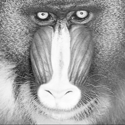
We also import the well known mandrill raster image.
from gridr.core.grid.grid_resampling import array_grid_resampling
from gridr.misc.mandrill import mandrill
Please note the mandrill image has 3 color’s channels.
Here we limit the image to the first channel and convert its type to 64 bits floating points.
image = mandrill[0]
grid_dtype = np.float64
data_in_dtype = np.float64
data_out_dtype = np.float64

array_in = image.astype(data_in_dtype)
Identity grid transform
We start by defining the idendity transform grid.
That’s not really impressive but we will go further to illustrate some variants (windowing, zooming, …)
Let’s first create the idendity transformation grid.
# create identity grid
if image.ndim == 2:
    x = np.arange(0, image.shape[0], dtype=grid_dtype)
    y = np.arange(0, image.shape[1], dtype=grid_dtype)
xx, yy = np.meshgrid(x, y)
Simple idendity transform
The array_grid_resampling method provides the array_out argument in order to use a preallocated C-contiguous array as output. It is quite convenient when implementing a tiling chain that uses that method.
For now, we choose to keep it simple : by setting array_out to None we let the method allocate the output buffer for us.
We have defined the rows and columns grids to be at full resolution, ie. there is one coordinate in the grids for each pixel in the input image. To stay at that resolution we set grid_resolution to 1 in both directions.
The array_grid_resampling function returns a tuple of two NumPy arrays. For now, we will focus on the first one — it contains the allocated output buffer, which holds the result of the interpolation.
For the interpolation method, we will primarily use the cubic identifier, which refers to the Optimized Bicubic interpolation algorithm. Other available interpolators include nearest, linear, bspline3, bspline5, bspline7, bspline9, and bspline11.
Note that the B-spline interpolators require additional parameters, which are detailed further in this guide within the masking section.
# Lets call the grid resampling
array_out_id, _ = array_grid_resampling(
        interp="cubic",
        array_in=image.astype(data_in_dtype),
        grid_row=yy,
        grid_col=xx,
        grid_resolution=(1,1),
        array_out=None,
        win=None,
        array_in_mask=None,
        grid_mask=None,
        array_out_mask=None,
        nodata_out=None,
        array_in_origin=None,
        )
In the following test we compare input with output. It must succeed !
np.testing.assert_almost_equal(array_in, array_out_id, decimal=10)
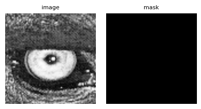
Apply a window
The array_grid_resampling method provides the win parameter in order to set a window to limit the region to compute.
The indices used in the win definition refers to indices considering the full resolution output.
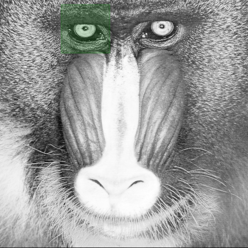
Below, we first define a window centered on the mandrill’s left eye. Since we are considering an identity grid, the grid coordinates align with the input array’s image coordinates
win_center = np.array((58, 175)) # left eye
win_shape =  np.array((100, 100))
win = np.array((win_center - win_shape//2, win_center - win_shape//2 + win_shape - 1)).T
array_out_id_win_1_1, _ = array_grid_resampling(
        interp="cubic",
        array_in=array_in,
        grid_row=yy,
        grid_col=xx,
        grid_resolution=(1,1),
        array_out=None,
        win=win,
        array_in_mask=None,
        grid_mask=None,
        array_out_mask=None,
        nodata_out=None,
        )

Playing with resolution to apply a zoom
The array_grid_resampling method uses the grid_resolution parameter to insert additional nodes between existing grid nodes. This insertion is achieved through bilinear interpolation, with the oversampling factors for both rows and columns specified in the grid_resolution parameter.
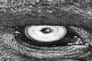
While the primary purpose of the grid_resolution is to control computation time and grid storage, in this case, we use it to perform a zoom operation, increasing the row resolution by a factor of 2 and the column resolution by a factor of 5.
At the same time, we want to maintain the same input region as before. To achieve this, the window definition must be adjusted to accommodate the new full-resolution output.
# Set resolution to the target zoom factors
resolution = (2, 3)

# The full resolution grid has (Nrow-1)*resolution_row + 1 rows (apply same logic on column)
full_output_shape = (np.asarray(array_in.shape) - 1)*resolution + 1

# setting output window to only consider a region of interest
# here we construct a window centered on the left eye in the full resolution output grid
win_center = np.array((58, 175)) * np.array(resolution)
win_shape =  np.array((100, 100)) * np.array(resolution)

win = np.array((win_center - win_shape//2, win_center - win_shape//2 + win_shape - 1)).T

# Lets call the grid resampling
array_out_id_zoom_2_5, _ = array_grid_resampling(
        interp="cubic",
        array_in=array_in,
        grid_row=yy,
        grid_col=xx,
        grid_resolution=resolution,
        array_out=None,
        win=win,
        array_in_mask=None,
        grid_mask=None,
        array_out_mask=None,
        nodata_out=None,
        )

In order to illustrate the change of interpolation method, we will use here the nearest identifier in order to adress a nearest neighbor interpolation.
# Lets call the grid resampling
array_out_id_zoom_2_5_nearest, _ = array_grid_resampling(
        interp="nearest",
        array_in=array_in,
        grid_row=yy,
        grid_col=xx,
        grid_resolution=resolution,
        array_out=None,
        win=win,
        array_in_mask=None,
        grid_mask=None,
        array_out_mask=None,
        nodata_out=None,
        )

# Let's show it
plot_im(array_out_id_zoom_2_5_nearest, None, prefix='004_nearest')
Geometry transformation examples
In that part we provide some examples of simple non identity transformation.
Translation transform
Let’s begin with a simple translation on the column coordinates by shifting the image to the left.
# First create identity grid
if image.ndim == 2:
    x = np.arange(0, image.shape[0], dtype=grid_dtype)
    y = np.arange(0, image.shape[1], dtype=grid_dtype)
xx, yy = np.meshgrid(x, y)
xx += 50.5

# Lets call the grid resampling
array_out_translation_left, _ = array_grid_resampling(
        interp="cubic",
        array_in=array_in,
        grid_row=yy,
        grid_col=xx,
        grid_resolution=(1,1),
        array_out=None,
        win=None,
        array_in_mask=None,
        grid_mask=None,
        array_out_mask=None,
        nodata_out=None,
        )
array_out_translation_left[:, -53:]
array([[124.875 ,      nan,      nan, ...,      nan,      nan,      nan],
       [130.    ,      nan,      nan, ...,      nan,      nan,      nan],
       [102.8125,      nan,      nan, ...,      nan,      nan,      nan],
       ...,
       [102.5625,      nan,      nan, ...,      nan,      nan,      nan],
       [ 86.5625,      nan,      nan, ...,      nan,      nan,      nan],
       [  3.5625,      nan,      nan, ...,      nan,      nan,      nan]],
      shape=(512, 53))
As you can see, the right strip border is filled with NaN values. It is due to the fact that the grid target coordinates went outside of the image’s definition domain.
Please note that the filling with NaN is not the default behaviour and it occured because we set the nodata_out parameter to None.
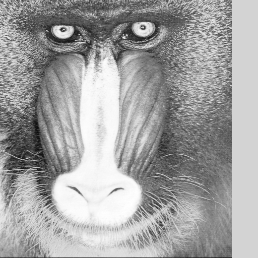
Let’s replay it by setting nodata_out to its default value, ie 0.
As you will see, the right strip border is now filled with zeros.
We also take this opportunity to introduce the use of the array_mask_out parameter and examine the second array returned by the function. We will verify that the mask correctly matches the nodata region of the resampled image. Here we set the array_out_mask parameter to True ; that’s a convenient way to let the array_grid_resampling method allocate the right sized unsigned byte (ie. uint8) array and return it. Please note that we can also directly pass a preallocated array similarly to the array_out parameter.
array_out_translation_left, array_out_translation_left_mask = array_grid_resampling(
        interp="cubic",
        array_in=array_in,
        grid_row=yy,
        grid_col=xx,
        grid_resolution=(1,1),
        array_out=None,
        win=None,
        array_in_mask=None,
        grid_mask=None,
        array_out_mask=True,
        nodata_out=0.,
        )
array_out_translation_left[:, -53:]
array([[124.875 ,   0.    ,   0.    , ...,   0.    ,   0.    ,   0.    ],
       [130.    ,   0.    ,   0.    , ...,   0.    ,   0.    ,   0.    ],
       [102.8125,   0.    ,   0.    , ...,   0.    ,   0.    ,   0.    ],
       ...,
       [102.5625,   0.    ,   0.    , ...,   0.    ,   0.    ,   0.    ],
       [ 86.5625,   0.    ,   0.    , ...,   0.    ,   0.    ,   0.    ],
       [  3.5625,   0.    ,   0.    , ...,   0.    ,   0.    ,   0.    ]],
      shape=(512, 53))
Let’s display the output validity mask
array_out_translation_left_mask[:, -53:]
array([[1, 0, 0, ..., 0, 0, 0],
       [1, 0, 0, ..., 0, 0, 0],
       [1, 0, 0, ..., 0, 0, 0],
       ...,
       [1, 0, 0, ..., 0, 0, 0],
       [1, 0, 0, ..., 0, 0, 0],
       [1, 0, 0, ..., 0, 0, 0]], shape=(512, 53), dtype=uint8)
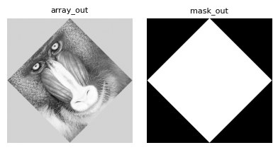
Rotation transform
Here we define a grid in order to apply a 45 degree rotation.
In order to have the full image rotated please note that we have to extend the grid size.
center = np.asarray(array_in.shape) // 2
theta = np.pi/4.
# we know the image is square - here we extend the output grid in order to cover
# the full image
ext = image.shape[0] * (2**0.5 - 1) // 2

# First create identity grid
if image.ndim == 2:
    x = np.arange(0, image.shape[0] + 2 * ext, dtype=grid_dtype) - ext
    y = np.arange(0, image.shape[1] + 2 * ext, dtype=grid_dtype) - ext
xx, yy = np.meshgrid(x , y)
# Apply the rotation
xrot = (xx - center[1]) * np.cos(theta) - (yy - center[0]) * np.sin(theta) + center[1]
yrot = (xx - center[1]) * np.sin(theta) + (yy - center[0]) * np.cos(theta) + center[0]
As a demonstration purpose we here preallocate the array_out buffer.
# We have to init the out buffer with the right shape
array_out = np.zeros(xx.shape, dtype=data_out_dtype)

# Lets call the grid resampling
_, mask_out = array_grid_resampling(
        interp="cubic",
        array_in=array_in,
        grid_row=yrot,
        grid_col=xrot,
        grid_resolution=(1,1),
        array_out=array_out,
        win=None,
        array_in_mask=None,
        grid_mask=None,
        array_out_mask=True,
        nodata_out=None,
        )
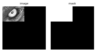
Specifying an output target window
In the previous step we opt to pre-allocate the output buffer for the image. What if the requested production window is smaller that the array_out buffer ?
# Set a window to focus on the left eye (we get the coordinates from the previous resampled image)
win = np.asarray([[250, 320], [120, 220]])

# We have to init the out buffer with an sufficient shape
array_out = np.zeros((200, 200), dtype=data_out_dtype)

# Lets call the grid resampling
_, mask_out = array_grid_resampling(
        interp="cubic",
        array_in=array_in,
        grid_row=yrot,
        grid_col=xrot,
        grid_resolution=(1,1),
        array_out=array_out,
        win=win,
        array_in_mask=None,
        grid_mask=None,
        array_out_mask=True,
        nodata_out=None,
        )
It’s worth noting that even without passing a preallocated output validity mask, the internally generated one will still match the shape of the array_out buffer.
As shown above, the resampled window is written starting at the origin of array_out (i.e., at [0, 0]).
In some cases - for example, when working with tiles that share a common output buffer - it may be necessary to write the result to a specific region within array_out.
This is precisely the purpose of the array_out_win parameter.
# Set a window to focus on the left eye (we get the coordinates from the previous resampled image)
win = np.asarray([[250, 320], [120, 220]])

# We have to init the out buffer with an sufficient shape
# Here we will also demonstrate that the resampling only modify the target window
# For that purpose we do not initialize with zeros but with arange
array_out = np.arange(200*200, dtype=data_out_dtype).reshape((200, 200)) % 255

# We also preallocate the validity mask for the same purpose
mask_out = np.arange(array_out.size, dtype=np.uint8).reshape(array_out.shape) % 10

# Let's define where we want to place the resampled window
array_out_win_origin = np.asarray([25, 40])
array_out_win = np.asarray([
    [array_out_win_origin[0], array_out_win_origin[0] + win[0][1] - win[0][0]],
    [array_out_win_origin[1], array_out_win_origin[1] + win[1][1] - win[1][0]]])


# Lets call the grid resampling
_, _ = array_grid_resampling(
        interp="cubic",
        array_in=array_in,
        grid_row=yrot,
        grid_col=xrot,
        grid_resolution=(1,1),
        array_out=array_out,
        array_out_win=array_out_win, # <= new parameter
        win=win,
        array_in_mask=None,
        grid_mask=None,
        array_out_mask=mask_out,
        nodata_out=None,
        )
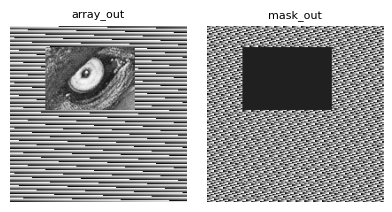
Note that this example also demonstrates that operating on a specific window only affects the corresponding region in the output array, leaving all other areas unchanged.
Working with masks
In this part we will see how to use masking.
The array_grid_resampling method provides several kind of masking for both the grid and the input array.
General convention
GridR resampling functionalities uses the following convention for mask :
the mask are considered unsigned 8 bits integers taking value in {0, 1}.
a value of 0 is considered as non valid
a value of 1 is considered as valid
Grid masking
Grid masking with a raster mask
Here we use an 8 bit raster having the same shape of the grids in order to devalidate points in the grid.
To keep it simple we will demonstrate using an identity transform.
# First create identity grid
if image.ndim == 2:
    x = np.arange(0, image.shape[0], dtype=grid_dtype)
    y = np.arange(0, image.shape[1], dtype=grid_dtype)
xx, yy = np.meshgrid(x, y)
We define the mask as following :
the first 10 lines and last 20 lines are masked
the first 30 columns and last 40 columns are masked
a 80x80 window positionned at the grid center are masked
Please note the mask applies to the grid and not to the input image.
By convention, the mask is considered binary. A value of 0 corresponds to a masked cell, a value of 1 corresponds to a valid cell.
# setting a mask to devalidate margins and center
grid_mask_valid_value = 1
grid_mask_invalid_value = 0
# the final multiplication here is not necessary but we keep it to show the mechanic
grid_mask = np.ones(xx.shape, dtype=np.uint8) * grid_mask_valid_value
# masked pixels are positiv ones
grid_mask[0:10] = grid_mask_invalid_value
grid_mask[-20:] = grid_mask_invalid_value
grid_mask[:,0:30] = grid_mask_invalid_value
grid_mask[:,-40:] = grid_mask_invalid_value
# devalidate center
grid_mask[image.shape[0]//2-40:image.shape[0]//2+40, image.shape[1]//2-40:image.shape[1]//2+40] = grid_mask_invalid_value
The nodata_out is used to set the output value affected by the masking operation.
# Lets call the grid resampling
array_out, mask_out = array_grid_resampling(
        interp="cubic",
        array_in=array_in,
        grid_row=yy,
        grid_col=xx,
        grid_resolution=(1,1),
        array_out=None,
        win=None,
        array_in_mask=None,
        grid_mask=grid_mask,
        grid_mask_valid_value=grid_mask_valid_value,
        array_out_mask=True,
        nodata_out=0,
        )
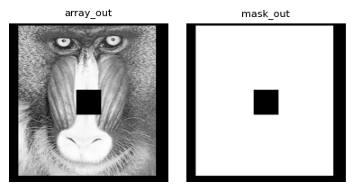
As in the previous example, we pass True to the function to obtain the validity mask output. We then check that it aligns correctly with the grid mask.
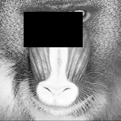
Masking with an inplaced grid nodata value
In this case, we avoid providing an additional mask, primarily to limit memory usage.
The array_grid_resampling method allows specifying a grid_nodata parameter, which is used to invalidate grid cells.
Cells in the grid whose values match this nodata value (within a fixed absolute tolerance of 1e-5) are treated as masked.
Providing a non-None value for grid_nodata activates the masking mechanism.
Note that it is not necessary to assign the nodata value to both grid coordinate arrays (row and column); setting it in either one is sufficient for the corresponding cell to be considered masked.
# Set a nodata value
grid_nodata = -999.
# Apply it to a window of the grid
yy[50:200,100:350] = grid_nodata
# Lets call the grid resampling
# Spoiler alert: this will fail !
try:
    array_out, _ = array_grid_resampling(
            interp="cubic",
            array_in=array_in,
            grid_row=yy,
            grid_col=xx,
            grid_resolution=(1,1),
            array_out=None,
            win=None,
            array_in_mask=None,
            grid_nodata=grid_nodata,
            grid_mask=grid_mask,
            grid_mask_valid_value=grid_mask_valid_value,
            array_out_mask=None,
            nodata_out=0,
            )
except ValueError as e:
    display(e)
ValueError('Only one of `grid_mask` or `grid_nodata` may be provided, not both.')
The call failed, and the ValueError exception provides the reason: both masking modes, grid_mask and grid_nodata, cannot be used simultaneously.
# Lets remove the grid_mask parameter's definition
array_out, _ = array_grid_resampling(
        interp="cubic",
        array_in=array_in,
        grid_row=yy,
        grid_col=xx,
        grid_resolution=(1,1),
        array_out=None,
        win=None,
        array_in_mask=None,
        grid_nodata=grid_nodata,
        grid_mask=None,
        grid_mask_valid_value=None,
        array_out_mask=None,
        nodata_out=0,
        )
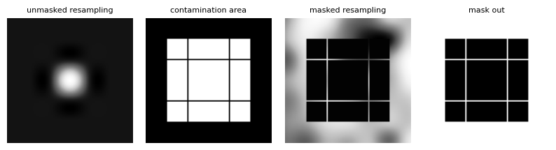
Effect of Grid Resolution on Grid Masking
Both the raster mask and the invalid_value grid mask remain consistent with the sampling of the grid.
When the resolution differs from 1 in a given direction, interpolation must occur within each grid cell — that is, within the mesh defined by four neighboring grid nodes. In such cases, if at least one non-zero weighted node of the mesh is masked, the interpolated result is marked as invalid. This results in nodata values in the resampled image and corresponding invalid entries (value 0) in the output mask.
Let’s illustrate this behavior by zooming in on a small region.
# create identity grid on the eye
if image.ndim == 2:
    x = np.arange(130, 220, dtype=grid_dtype)
    y = np.arange(30, 100, dtype=grid_dtype)
xx, yy = np.meshgrid(x, y)

resolution = np.asarray((2,3))

# lets define the mask using grid_nodata
grid_nodata = -99999
yy[30, 35] = grid_nodata

array_out, mask_out = array_grid_resampling(
        interp="cubic",
        array_in=array_in,
        grid_row=yy,
        grid_col=xx,
        grid_resolution=tuple(resolution),
        array_out=None,
        win=None,
        array_in_mask=None,
        grid_nodata=grid_nodata,
        array_out_mask=True,
        nodata_out=0,
        )
To invalidate a specific grid position, we’ve configured the input (30, 35). This grid coordinate directly corresponds to the (60, 105) output position in the output coordinate system.
print(mask_out[60-2:60+3,105-3:105+4])
print(f"Number of masked data : {np.where(mask_out==0)[0].shape}")
[[1 1 1 1 1 1 1]
 [1 0 0 0 0 0 1]
 [1 0 0 0 0 0 1]
 [1 0 0 0 0 0 1]
 [1 1 1 1 1 1 1]]
Number of masked data : (15,)
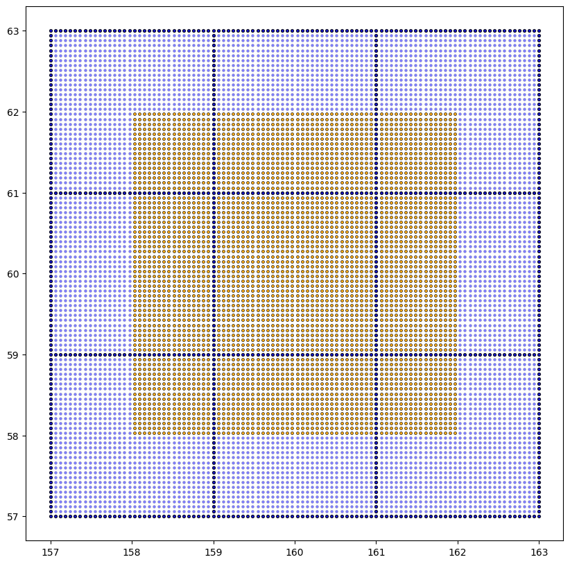
The masked area, as illustrated, exceeds a single pixel due to a resolution factor of 2 for rows and 3 for columns. The displayed array is centered on the position of the invalid grid node. Notably, this invalidation propagates to its immediate neighborhood, but exclusively for interpolated values where its weight is non-zero.
For clearer comprehension, in the schema below, an x denotes an invalid grid node, an o represents other grid nodes, and both - and * signify oversampled positions. It’s crucial to note that only the * positions utilize the x (invalid grid node) in their bilinear interpolation calculations.
 o - - o - - o
 - * * * * * -
 o * * x * * o
 - * * * * * -
 o - - o - - o
Input Array masking
Array masking with a raster mask
Here we use an 8 bit raster having the same shape of the input array in order to devalidate points in the input array.
Basically if input data is devalidate, interpolation that involves those data must be considered as not valid resulting in output valued to nodata_out and the optional array_out_mask set to 0 instead of 1.
To keep it simple we will demonstrate using a simple zoom transformation transform.
array_in_mask = np.ones(array_in.shape, dtype=np.uint8)
masked_pos = (60, 160)
array_in_mask[*masked_pos] = 0
# In order to check the good interpolation we will also set the array_in to hold an aberrant value
save_array_in = array_in[*masked_pos]

# Create a grid centered on the masked position
y = masked_pos[0] + np.linspace(-3, 3, 100)
x = masked_pos[1] + np.linspace(-3, 3, 100)
xx, yy = np.meshgrid(x, y)

# First compute a reference
array_out_womask_truth, _ = array_grid_resampling(
        interp="cubic",
        array_in=array_in,
        grid_row=yy,
        grid_col=xx,
        grid_resolution=(1,1),
        array_out=None,
        nodata_out=0,
        )

# Second compute without array masking to watch the effect of the non masked aberrant value
array_in[*masked_pos] = 1e7

array_out_womask, _ = array_grid_resampling(
        interp="cubic",
        array_in=array_in,
        grid_row=yy,
        grid_col=xx,
        grid_resolution=(1,1),
        array_out=None,
        array_out_mask=True,
        nodata_out=0,
        )

aberrant_radiation = np.zeros(array_out_womask.shape)
aberrant_radiation[np.where(array_out_womask - array_out_womask_truth != 0)] = 1

# Recompute with the mask
array_out, mask_out = array_grid_resampling(
        interp="cubic",
        array_in=array_in,
        grid_row=yy,
        grid_col=xx,
        grid_resolution=(1,1),
        array_in_mask=array_in_mask,
        array_out=None,
        array_out_mask=True,
        nodata_out=150, # Here we set nodata_out to 150 in order to have some texture for the display
        )
# restore array_in
array_in[*masked_pos] = save_array_in
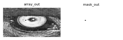
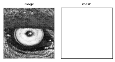
We have several plots to analyze here.
The first plot reveals what happens when the anomalous value is not masked. While the 8-bit display dynamic range prevents us from fully appreciating the valid interpolation, this plot effectively showcases the influence of an anomalous value (exaggerated for illustrative purposes) on the interpolation process.
The second plot, a binary representation, indicates where the anomalous value “spreads” or “irradiates.” Interestingly, some unaffected lines can be seen traversing the “irradiated” zone.
The third plot demonstrates the outcome when the anomalous value is successfully masked. We can see a clear correspondence between the no-data pixels and the “irradiated” area.
Lastly, the final plot presents the output validity mask, confirming its consistency with our earlier findings.
# min and max indices of masked data
upper_left = np.min(np.where(mask_out==0), axis=1)
lower_right = np.max(np.where(mask_out==0), axis=1)
print(f'upper left corner of masked data : {upper_left}')
print(f'lower right corner of masked data : {lower_right}')

# corresponding grid coordinates
print(f'masked data upper left corner grid coordinates : {yy[*upper_left], xx[*upper_left]}')
print(f'masked data lower right corner grid coordinates : {yy[*lower_right], xx[*lower_right]}')
upper left corner of masked data : [17 17]
lower right corner of masked data : [82 82]
masked data upper left corner grid coordinates : (np.float64(58.03030303030303), np.float64(158.03030303030303))
masked data lower right corner grid coordinates : (np.float64(61.96969696969697), np.float64(161.96969696969697))
The optimized bicubic interpolator uses a spatial support of ±2 around the target coordinates. This directly explains the masked area’s boundaries: row indices [58,62] and column indices [158,162].
Now, let’s discuss the unmasked lines that cross the invalid area. To do this, we will plot the grid coordinates, differentiating between the valid and invalid ones.
We’ve used a distinct style in the plot above to highlight coordinates that fall on exact integer values. This specific scenario, where we have whole integer coordinates within our grid, serves to prove that the GridR implementation aligns correctly with the “irradiated” area. It also shows that it avoids inadvertently masking pixels that should remain unmasked.
What makes these integer coordinate positions unique? For these particular points, the subsequent interpolation process can utilize a directly available value in at least one direction, meaning no actual interpolation is required along that axis. In these instances, the neighboring points that would normally contribute to the interpolation—especially any anomalous ones—are effectively bypassed. Their associated coefficients are set to zero, which then yields a perfectly valid interpolated value.
Masking with a Cardinal B-Spline Interpolator
GridR implements Cardinal B-spline interpolation based on [1]. While we won’t detail their algorithms here, we focus on GridR’s unique mask handling features not covered in the original paper.
The interpolation process requires both causal and anti-causal recursive prefiltering applied to the input image. While these filters theoretically require infinite sums, GridR approximates them using finite sums as proposed in the reference article. This approximation relies on either the image’s immediate neighborhood or extrapolated data through boundary conditions (detailed further below).
The recursive filters used in B-spline interpolation exhibit an exponential decay property. When a pixel is invalid, its influence propagates to neighboring pixels through the recursive filtering process, but this influence decreases exponentially with distance. For a pole \(z_k\) (where \(-1 < z_k < 0\)), the exponential filter has the form:
This shows that the 1D influence at distance \(j\) pixels decays as \(|z_k|^{|j|}\).
In practice, the dominant pole (largest absolute value, typically \(z_1\)) determines the decay rate. To determine at what distance \(d\) the 1D influence becomes negligible, we solve:
where \(d\) is the distance in pixels and \(s\) is the acceptable residual influence threshold.
This gives:
Since the prefiltering is performed separably on rows and column, the 2D influence can be expressed as :
In the 2D case we then have to consider the Manhattan distance (not Euclidian). In practice, this yields a diamond-shaped (45° oriented square) influence zone centered around the invalid pixel’s position.
Instead of filtering the validity mask (which can produce overshoots artifacts), a more robust approach is to dilate the invalid area within the validity mask by the computed influence radius using a Manhattan distance structuring element.
Additionally, mask elements corresponding to image pixels used to approximate the infinite sums - refered as domain extension in the article - are automatically invalidated during the mask prefiltering process. This invalidation occurs after the previously mentioned propagation of invalid mask elements.
It is important to note that the residual influence threshold \(s\) is relative to the invalid pixel value itself. For extreme outlier values (e.g. contaminated pixel with 10000 in a 0-255 image), even a small relative threshold (e.g., \(s = 10^{-3} = 0.1%\)) can correspond to a significant absolute contamination (\(10000 \times 10^{-3} = 10\)), requiring a much larger dilatation radius than for typical data values. When dealing with aberrant values, the threshold \(s\) should be chosen accodingly to ensure the absolute contamination remains acceptable for your application.
Let’s examine how GridR handles masking for B-spline prefiltering. Additionnaly we will notice we need to pass two additional arguments for B-spline interpolation: epsilon and mask_influence_threshold.
The epsilon parameter defines the acceptable error when approximating the finite sums, directly affecting the required margins for prefiltering on each side (referred to as truncation index in the reference article). For a fixed B-spline order, the smaller this value, the larger the required margin becomes. Note that the total required margin is the sum of both the prefiltering margin and the margin needed for pure interpolation, corresponding to the interpolation kernel radius.
The mask_influence_threshold parameter is particularly important here and corresponds to the the residual influence threshold \(s\) previously mentioned.
We now demonstrate how an aberrant point propagates through both the image and validity mask, comparing results with and without GridR’s specialized B-spline prefiltering mask handling.
# Create a grid centered on the masked position
# Here we use a larger input domain as previously in order to demonstrate the
# behaviour of prefiltering.
zoom = 4
y = masked_pos[0] + np.linspace(-20, 20, 40*zoom+1)
x = masked_pos[1] + np.linspace(-20, 20, 40*zoom+1)
xx, yy = np.meshgrid(x, y)

# We will use the same input as before but we need to copy it as the B-spline
# prefiltering will operate in place.
array_in_truth = np.copy(array_in)

# First compute resampling with all valid data without altering
# the element going to be invalid
array_out_womask_truth, array_mask_out_womask_truth = array_grid_resampling(
        interp="bspline3",
        interp_kwargs={"epsilon": 1e-6, "mask_influence_threshold": 1},
        array_in=array_in_truth,
        grid_row=yy,
        grid_col=xx,
        grid_resolution=(1,1),
        array_out=None,
        array_out_mask=True,
        nodata_out=0,
        )

# Perform a second computation after making the target element aberrant,
# without activating array masking, to observe how the unmasked aberrant
# value affects the result.
anomalous_value = 1e9
array_in_womask = np.copy(array_in)
array_in_womask[*masked_pos] = anomalous_value

array_out_womask, array_mask_out_womask = array_grid_resampling(
        interp="bspline3",
        interp_kwargs={"epsilon": 1e-6, "mask_influence_threshold": 1},
        array_in=array_in_womask,
        grid_row=yy,
        grid_col=xx,
        grid_resolution=(1,1),
        array_out=None,
        array_out_mask=True,
        nodata_out=0,
        )

# For plot purpose we will set to nodata values that differs more than 1
# in absolute value from the reference output
ref_masked = np.abs(array_out_womask - array_out_womask_truth) > 1
array_out_womask_custom = np.copy(array_out_womask)
array_out_womask_custom[ref_masked] = 0
/tmp/ipykernel_3950/3703061842.py:3: RuntimeWarning: invalid value encountered in log
  'wo_in_mask_log': np.log(array_out_womask),
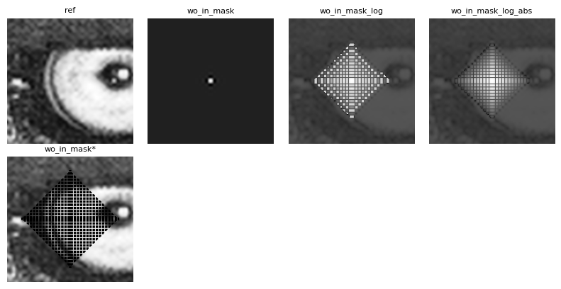
Once more we have several plots to comment. From left to right,
The first plot corresponds to a reference resampling with no abberation at all.
The second plot shows the resampling result after modifying the input data to create an aberrant center element. While we can observe some propagation of this aberrant point, the extreme value (\(10^9\) - exaggerated for demonstration purposes) makes it impossible to display the result’s full dynamic range using linear scaling in an 8-bit grayscale format. Thus motivating the next plot.
The third plot shows the same data than the previous one but using a logarithm scaling for display. It clearly shows the propagation of the aberration while making it possible to guess the region were the image is valid. You can also notice oscillation within the propagation area: they are caracterial of prefiltering around a disruptive point - negative values are here showed as NaN explaining why the same gray color is used for all of them.
The fourth plot comes as complement of the third one. Here it shows the same data but using a logarithm scaling on its absolute value for display. This serves as observing the exponential decay of the influence of the anomalous value.
The last plot shows the same result data but this time the pixels whose value differs from the reference of 0.1 are masked out for display. While the value of 0.1 is arbitrary, we can experimentally check the obtained distance for the corresponding threshold \(s = 0.1 * 1e^{-9} = 1e^{-10}\).
# Experienced distance - compute it from vertical diameter and considering the zoom_factor (4x)
zoom = 1. / (y[1]-y[0])
left = np.min(np.where(ref_masked == 1)[0])
right = np.max(np.where(ref_masked == 1)[0])
d = (right - left) / (2 * zoom)
print(f"Measured influence distance : {d}")

# Theoretical distance
bspline3_z1 = -2.679491924311227e-1
d_th = np.log(1./anomalous_value) / np.log(np.abs(bspline3_z1))
print(f"Theretical influence distance : {d_th}")
Measured influence distance : 15.5
Theretical influence distance : 15.735708700586859
An interesting point observed in the last plot is that, since the grid performs an exact 4x zoom, every fourth point targets a whole source coordinate. For these points, the interpolated values are not contaminated by aberrant values.
Let’s now examine how GridR handles masks by activating the usage of an input mask. We set the mask_influence_threshold parameter such that the absolute residual does not exceed a value of 1, aligning with the previously obtained experimental masking. Since this threshold is relative to the anomalous value, we set it to \(1. / 10^{-9} = 10^{-10}\), resulting in a computed distance of 15.73 as shown earlier.
# Perform a computation after making the target element aberrant,
# with activating array masking
array_in_wmask_mask = np.ones(array_in.shape, dtype=np.uint8)
array_in_wmask_mask[*masked_pos] = 0

# Copy mask as it will be updated in place
array_in_wmask = np.copy(array_in)
array_in_wmask[*masked_pos] = anomalous_value

# Here we set mask_influence_threshold to match the targeted accepted
# residual of the anomalous value.
# We want it to correspond to 0.1 in absolute value
array_out_wmask, array_mask_out_wmask = array_grid_resampling(
        interp="bspline3",
        interp_kwargs={"epsilon": 1e-6, "mask_influence_threshold": 1./anomalous_value},
        array_in=array_in_wmask,
        array_in_mask=array_in_wmask_mask,
        grid_row=yy,
        grid_col=xx,
        grid_resolution=(1,1),
        array_out=None,
        array_out_mask=True,
        nodata_out=0,
        )

array_out_wmask_masked = np.copy(array_out_wmask)
array_out_wmask_masked[array_mask_out_wmask == 0] = 0
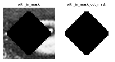
In this case, the diamond-shaped mask is internally computed during the prefiltering stage and subsequently used as an updated mask for the interpolation process. Consequently, any invalid data within the mask are automatically set to the nodata value specified through the nodata_out parameter.
Boundary condition
In this section, we will examine what occurs when interpolating data at the boundaries of the source array. To focus on a specific region of interest, we will crop the source array and store the relevant portion in a new buffer.
win_center = np.array((58, 175)) # left eye
win_shape =  np.array((80, 80))
win = np.array((win_center - win_shape//2, win_center - win_shape//2 + win_shape - 1)).T

array_in_cropped = np.empty(win_shape, dtype=array_in.dtype, order='C')
array_in_cropped[:] = array_in[win[0][0]:win[0][1]+1, win[1][0]:win[1][1]+1]

We generate an identity grid that spans the entire domain of the source image. By utilizing the resolution parameter, we apply a zoom factor of 4x.
# First create identity grid
zoom = 4
if image.ndim == 2:
    x = np.arange(0, array_in_cropped.shape[0], dtype=grid_dtype)
    y = np.arange(0, array_in_cropped.shape[1], dtype=grid_dtype)
xx, yy = np.meshgrid(x, y)

# Lets call the grid resampling
array_out_cropped_zoom, array_out_cropped_zoom_mask = array_grid_resampling(
        interp="cubic",
        array_in=array_in_cropped,
        grid_row=yy,
        grid_col=xx,
        grid_resolution=(zoom,zoom),
        array_out=None,
        win=None,
        array_in_mask=None,
        grid_mask=None,
        array_out_mask=True,
        nodata_out=None,
        )
We have just performed a 4x zoom in both directions using a cubic interpolator. This interpolator has a radius of 2, which means that when interpolating near the edges of the image, it needs to access positions outside the source image domain.
# Left output edge
np.round(array_out_cropped_zoom[4:9, 0:7], 2), array_out_cropped_zoom_mask[4:9, 0:7]
(array([[127.  ,    nan,    nan,    nan, 118.  , 102.01,  79.31],
        [118.77,    nan,    nan,    nan, 116.18, 101.47,  80.01],
        [107.62,    nan,    nan,    nan, 116.44, 103.69,  83.93],
        [ 96.67,    nan,    nan,    nan, 115.73, 105.36,  88.05],
        [ 89.  ,    nan,    nan,    nan, 111.  , 103.18,  89.31]]),
 array([[1, 0, 0, 0, 1, 1, 1],
        [1, 0, 0, 0, 1, 1, 1],
        [1, 0, 0, 0, 1, 1, 1],
        [1, 0, 0, 0, 1, 1, 1],
        [1, 0, 0, 0, 1, 1, 1]], dtype=uint8))
As observed, the cubic interpolator returns NaN (the value set for nodata_out) for output column indexes 1, 2, and 3. These indexes correspond to source column positions at 0.25, 0.5, and 0.75, respectively. The interpolation requires accessing column values at the source’s negative column position -1, which is not available. This invalidates the output mask for these positions, resulting in NaN values in the output image.
To address these edge cases, the boundary_condition parameter (default = None) can be set. This parameter handles scenarios where the interpolation requires positions outside the source image domain. The accepted values are a subset of the numpy.pad accepted values for the mode parameter, including:
‘edge’: Pad with the edge values of the array (repeat boundary values).
‘wrap’: Wrap around to the opposite edge (circular/periodic boundary).
‘reflect’: Mirror reflection without repeating the edge values.
‘symmetric’: Mirror reflection with edge values repeated.
It is important to note that when a boundary condition is applied, interpolated values are not systematically invalidated by the output mask. This is because the mask itself is subject to the same boundary condition, ensuring consistency in the handling of edge cases.
The boundary_condition parameter requires the standalone parameter to be set to True, which is the default value. We will explore this mode in more detail later.
Now, let’s apply a ‘reflect’ boundary condition and examine the effect on the output data.
# Lets call the grid resampling with a boundary condition
array_out_cropped_zoom_reflect, array_out_cropped_zoom_mask_reflect = array_grid_resampling(
        interp="cubic",
        array_in=array_in_cropped,
        grid_row=yy,
        grid_col=xx,
        grid_resolution=(zoom,zoom),
        array_out=None,
        win=None,
        array_in_mask=None,
        grid_mask=None,
        array_out_mask=True,
        nodata_out=None,
        boundary_condition="reflect",
        standalone=True,
        )
# Left output edge after reflect
np.round(array_out_cropped_zoom_reflect[4:9, 0:7], 2), array_out_cropped_zoom_mask_reflect[4:9, 0:7]
(array([[127.  , 127.4 , 127.31, 124.82, 118.  , 102.01,  79.31],
        [118.77, 119.96, 121.73, 121.37, 116.18, 101.47,  80.01],
        [107.62, 110.25, 115.36, 118.8 , 116.44, 103.69,  83.93],
        [ 96.67, 100.52, 108.52, 115.36, 115.73, 105.36,  88.05],
        [ 89.  ,  93.  , 101.5 , 109.25, 111.  , 103.18,  89.31]]),
 array([[1, 1, 1, 1, 1, 1, 1],
        [1, 1, 1, 1, 1, 1, 1],
        [1, 1, 1, 1, 1, 1, 1],
        [1, 1, 1, 1, 1, 1, 1],
        [1, 1, 1, 1, 1, 1, 1]], dtype=uint8))
As you can see, all output data is now valid and there are no more NaN values.
The standalone mode
Coming in the future…
Advanced Usage: Pipeline Integration (standalone=False)
Adjusting the Origin of Input Coordinates
The array_grid_resampling function includes the parameter array_in_origin (default: (0., 0.)) that allows shifting the origin of the input coordinate system.
From an implementation standpoint, this shift is applied directly to the computed target grid coordinates.
This feature is useful in several scenarios:
Handling different grid conventions without modifying the grid itself. As a reminder, GridR assumes that integer coordinates refer to pixel centers. In other systems, a pixel may be treated as an area, with its center located relatively at (0.5, 0.5).
Working with subregions of a larger input array. In this case, the shift can represent the position of the subregion within the full array’s coordinate system.
As an example we will take a previous example using an idendity transformation.
# create identity grid
if image.ndim == 2:
    x = np.arange(0, image.shape[0], dtype=grid_dtype)
    y = np.arange(0, image.shape[1], dtype=grid_dtype)
xx, yy = np.meshgrid(x, y)

win_center = np.array((58, 175)) # left eye
win_shape =  np.array((100, 100))
win = np.array((win_center - win_shape//2, win_center - win_shape//2 + win_shape - 1)).T

# Call it without specifying array_in_origin
array_out_origin_0_0, _ = array_grid_resampling(
        interp="cubic",
        array_in=array_in,
        grid_row=yy,
        grid_col=xx,
        grid_resolution=(1,1),
        array_out=None,
        win=win,
        array_in_mask=None,
        grid_mask=None,
        array_out_mask=None,
        nodata_out=None,
        )

# Call it with specifying array_in_origin and passing standalone=False
array_out_origin_30_m10, _ = array_grid_resampling(
        interp="cubic",
        array_in=array_in,
        array_in_origin=(30, -10), # <= shift +30 on rows and -10 on columns
        grid_row=yy,
        grid_col=xx,
        grid_resolution=(1,1),
        array_out=None,
        win=win,
        array_in_mask=None,
        grid_mask=None,
        array_out_mask=None,
        nodata_out=None,
        standalone=False,
        )
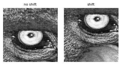
As you can observe, the coordinate shift is reflected in the bottom image.