Using the GridR’s core grid resampling API
This guide shows how to use the core array_grid_resampling GridR’s feature.
It covers the following topics:
Performing basic grid-based resampling
Working with spatial windows
Controlling output grid resolution
Handling nodata values and generating output validity masks
Moving the input data origin
Using masks to control the validity of input grids and input data
Setting things up
First we have to import the array_grid_resampling method.
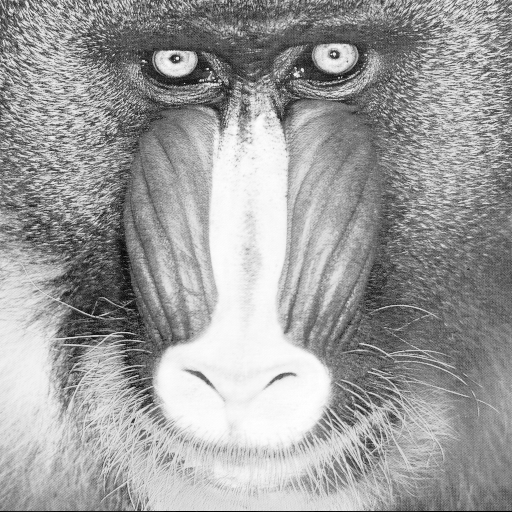
We also import the well known mandrill raster image.
from gridr.core.grid.grid_resampling import array_grid_resampling
from gridr.misc.mandrill import mandrill
Please note the mandrill image has 3 color’s channels.
Here we limit the image to the first channel and convert its type to 64 bits floating points.
image = mandrill[0]
grid_dtype = np.float64
data_in_dtype = np.float64
data_out_dtype = np.float64

array_in = image.astype(data_in_dtype)
Identity grid transform
We start by defining the idendity transform grid.
That’s not really impressive but we will go further to illustrate some variants (windowing, zooming, …)
Let’s first create the idendity transformation grid.
# create identity grid
if image.ndim == 2:
    x = np.arange(0, image.shape[0], dtype=grid_dtype)
    y = np.arange(0, image.shape[1], dtype=grid_dtype)
xx, yy = np.meshgrid(x, y)
Simple idendity transform
The array_grid_resampling method provides the array_out argument in order to use a preallocated C-contiguous array as output. It is quite convenient when implementing a tiling chain that uses that method.
For now, we choose to keep it simple : by setting array_out to None we let the method allocate the output buffer for us.
We have defined the rows and columns grids to be at full resolution, ie. there is one coordinate in the grids for each pixel in the input image. To stay at that resolution we set grid_resolution to 1 in both directions.
The array_grid_resampling function returns a tuple of two NumPy arrays. For now, we will focus on the first one — it contains the allocated output buffer, which holds the result of the interpolation.
For the interpolation method, we will employ the cubic identifier, which designates the Optimized Bicubic interpolation algorithm.
# Lets call the grid resampling
array_out_id, _ = array_grid_resampling(
        interp="cubic",
        array_in=image.astype(data_in_dtype),
        grid_row=yy,
        grid_col=xx,
        grid_resolution=(1,1),
        array_out=None,
        win=None,
        array_in_mask=None,
        grid_mask=None,
        array_out_mask=None,
        nodata_out=None,
        )
In the following test we compare input with output. It must succeed !
np.testing.assert_almost_equal(array_in, array_out_id, decimal=10)
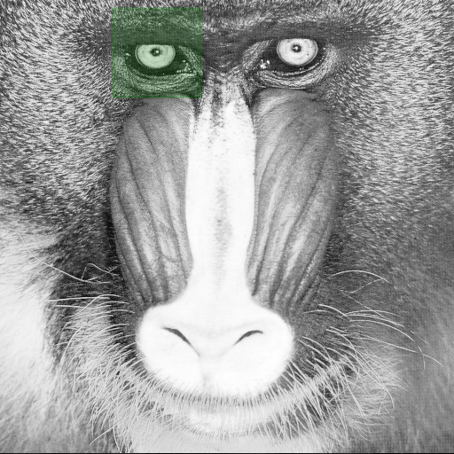
Apply a window
The array_grid_resampling method provides the win parameter in order to set a window to limit the region to compute.
The indices used in the win definition refers to indices considering the full resolution output.
Below, we first define a window centered on the mandrill’s left eye. Since we are considering an identity grid, the grid coordinates align with the input array’s image coordinates
win_center = np.array((58, 175)) # left eye
win_shape =  np.array((100, 100))
win = np.array((win_center - win_shape//2, win_center - win_shape//2 + win_shape - 1)).T
array_out_id_win_1_1, _ = array_grid_resampling(
        interp="cubic",
        array_in=array_in,
        grid_row=yy,
        grid_col=xx,
        grid_resolution=(1,1),
        array_out=None,
        win=win,
        array_in_mask=None,
        grid_mask=None,
        array_out_mask=None,
        nodata_out=None,
        )

Playing with resolution to apply a zoom
The array_grid_resampling method uses the grid_resolution parameter to insert additional nodes between existing grid nodes. This insertion is achieved through bilinear interpolation, with the oversampling factors for both rows and columns specified in the grid_resolution parameter.
While the primary purpose of the grid_resolution is to control computation time and grid storage, in this case, we use it to perform a zoom operation, increasing the row resolution by a factor of 2 and the column resolution by a factor of 5.
At the same time, we want to maintain the same input region as before. To achieve this, the window definition must be adjusted to accommodate the new full-resolution output.
# Set resolution to the target zoom factors
resolution = (2, 3)

# The full resolution grid has (Nrow-1)*resolution_row + 1 rows (apply same logic on column)
full_output_shape = (np.asarray(array_in.shape) - 1)*resolution + 1

# setting output window to only consider a region of interest
# here we construct a window centered on the left eye in the full resolution output grid
win_center = np.array((58, 175)) * np.array(resolution)
win_shape =  np.array((100, 100)) * np.array(resolution)

win = np.array((win_center - win_shape//2, win_center - win_shape//2 + win_shape - 1)).T

# Lets call the grid resampling
array_out_id_zoom_2_5, _ = array_grid_resampling(
        interp="cubic",
        array_in=array_in,
        grid_row=yy,
        grid_col=xx,
        grid_resolution=resolution,
        array_out=None,
        win=win,
        array_in_mask=None,
        grid_mask=None,
        array_out_mask=None,
        nodata_out=None,
        )
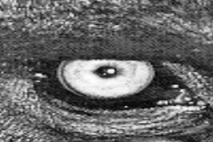
In order to illustrate the change of interpolation method, we will use here the nearest identifier in order to adress a nearest neighbor interpolation.
# Lets call the grid resampling
array_out_id_zoom_2_5_nearest, _ = array_grid_resampling(
        interp="nearest",
        array_in=array_in,
        grid_row=yy,
        grid_col=xx,
        grid_resolution=resolution,
        array_out=None,
        win=win,
        array_in_mask=None,
        grid_mask=None,
        array_out_mask=None,
        nodata_out=None,
        )

# Let's show it
plot_im(array_out_id_zoom_2_5_nearest, None, prefix='004_nearest')

Geometry transformation examples
In that part we provide some examples of simple non identity transformation.
Translation transform
Let’s begin with a simple translation on the column coordinates by shifting the image to the left.
# First create identity grid
if image.ndim == 2:
    x = np.arange(0, image.shape[0], dtype=grid_dtype)
    y = np.arange(0, image.shape[1], dtype=grid_dtype)
xx, yy = np.meshgrid(x, y)
xx += 50.5

# Lets call the grid resampling
array_out_translation_left, _ = array_grid_resampling(
        interp="cubic",
        array_in=array_in,
        grid_row=yy,
        grid_col=xx,
        grid_resolution=(1,1),
        array_out=None,
        win=None,
        array_in_mask=None,
        grid_mask=None,
        array_out_mask=None,
        nodata_out=None,
        )
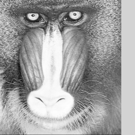
array_out_translation_left[:, -53:]
array([[124.875 ,      nan,      nan, ...,      nan,      nan,      nan],
       [130.    ,      nan,      nan, ...,      nan,      nan,      nan],
       [102.8125,      nan,      nan, ...,      nan,      nan,      nan],
       ...,
       [102.5625,      nan,      nan, ...,      nan,      nan,      nan],
       [ 86.5625,      nan,      nan, ...,      nan,      nan,      nan],
       [  3.5625,      nan,      nan, ...,      nan,      nan,      nan]],
      shape=(512, 53))
As you can see, the right strip border is filled with NaN values. It is due to the fact that the grid target coordinates went outside of the image’s definition domain.
Please note that the filling with NaN is not the default behaviour and it occured because we set the nodata_out parameter to None.
Let’s replay it by setting nodata_out to its default value, ie 0.
As you will see, the right strip border is now filled with zeros.
We also take this opportunity to introduce the use of the array_mask_out parameter and examine the second array returned by the function. We will verify that the mask correctly matches the nodata region of the resampled image. Here we set the array_out_mask parameter to True ; that’s a convenient way to let the array_grid_resampling method allocate the right sized unsigned byte (ie. uint8) array and return it. Please note that we can also directly pass a preallocated array similarly to the array_out parameter.
array_out_translation_left, array_out_translation_left_mask = array_grid_resampling(
        interp="cubic",
        array_in=array_in,
        grid_row=yy,
        grid_col=xx,
        grid_resolution=(1,1),
        array_out=None,
        win=None,
        array_in_mask=None,
        grid_mask=None,
        array_out_mask=True,
        nodata_out=0.,
        )
array_out_translation_left[:, -53:]
array([[124.875 ,   0.    ,   0.    , ...,   0.    ,   0.    ,   0.    ],
       [130.    ,   0.    ,   0.    , ...,   0.    ,   0.    ,   0.    ],
       [102.8125,   0.    ,   0.    , ...,   0.    ,   0.    ,   0.    ],
       ...,
       [102.5625,   0.    ,   0.    , ...,   0.    ,   0.    ,   0.    ],
       [ 86.5625,   0.    ,   0.    , ...,   0.    ,   0.    ,   0.    ],
       [  3.5625,   0.    ,   0.    , ...,   0.    ,   0.    ,   0.    ]],
      shape=(512, 53))
Let’s display the output validity mask
array_out_translation_left_mask[:, -53:]
array([[1, 0, 0, ..., 0, 0, 0],
       [1, 0, 0, ..., 0, 0, 0],
       [1, 0, 0, ..., 0, 0, 0],
       ...,
       [1, 0, 0, ..., 0, 0, 0],
       [1, 0, 0, ..., 0, 0, 0],
       [1, 0, 0, ..., 0, 0, 0]], shape=(512, 53), dtype=uint8)
Rotation transform
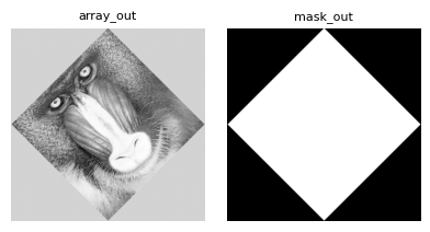
Here we define a grid in order to apply a 45 degree rotation.
In order to have the full image rotated please note that we have to extend the grid size.
center = np.asarray(array_in.shape) // 2
theta = np.pi/4.
# we know the image is square - here we extend the output grid in order to cover
# the full image
ext = image.shape[0] * (2**0.5 - 1) // 2

# First create identity grid
if image.ndim == 2:
    x = np.arange(0, image.shape[0] + 2 * ext, dtype=grid_dtype) - ext
    y = np.arange(0, image.shape[1] + 2 * ext, dtype=grid_dtype) - ext
xx, yy = np.meshgrid(x , y)
# Apply the rotation
xrot = (xx - center[1]) * np.cos(theta) - (yy - center[0]) * np.sin(theta) + center[1]
yrot = (xx - center[1]) * np.sin(theta) + (yy - center[0]) * np.cos(theta) + center[0]
As a demonstration purpose we here preallocate the array_out buffer.
# We have to init the out buffer with the right shape
array_out = np.zeros(xx.shape, dtype=data_out_dtype)

# Lets call the grid resampling
_, mask_out = array_grid_resampling(
        interp="cubic",
        array_in=array_in,
        grid_row=yrot,
        grid_col=xrot,
        grid_resolution=(1,1),
        array_out=array_out,
        win=None,
        array_in_mask=None,
        grid_mask=None,
        array_out_mask=True,
        nodata_out=None,
        )
Specifying an output target window
In the previous step we opt to pre-allocate the output buffer for the image. What if the requested production window is smaller that the array_out buffer ?
# Set a window to focus on the left eye (we get the coordinates from the previous resampled image)
win = np.asarray([[250, 320], [120, 220]])

# We have to init the out buffer with an sufficient shape
array_out = np.zeros((200, 200), dtype=data_out_dtype)

# Lets call the grid resampling
_, mask_out = array_grid_resampling(
        interp="cubic",
        array_in=array_in,
        grid_row=yrot,
        grid_col=xrot,
        grid_resolution=(1,1),
        array_out=array_out,
        win=win,
        array_in_mask=None,
        grid_mask=None,
        array_out_mask=True,
        nodata_out=None,
        )
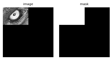
It’s worth noting that even without passing a preallocated output validity mask, the internally generated one will still match the shape of the array_out buffer.
As shown above, the resampled window is written starting at the origin of array_out (i.e., at [0, 0]).
In some cases - for example, when working with tiles that share a common output buffer - it may be necessary to write the result to a specific region within array_out.
This is precisely the purpose of the array_out_win parameter.
# Set a window to focus on the left eye (we get the coordinates from the previous resampled image)
win = np.asarray([[250, 320], [120, 220]])

# We have to init the out buffer with an sufficient shape
# Here we will also demonstrate that the resampling only modify the target window
# For that purpose we do not initialize with zeros but with arange
array_out = np.arange(200*200, dtype=data_out_dtype).reshape((200, 200)) % 255

# We also preallocate the validity mask for the same purpose
mask_out = np.arange(array_out.size, dtype=np.uint8).reshape(array_out.shape) % 10

# Let's define where we want to place the resampled window
array_out_win_origin = np.asarray([25, 40])
array_out_win = np.asarray([
    [array_out_win_origin[0], array_out_win_origin[0] + win[0][1] - win[0][0]],
    [array_out_win_origin[1], array_out_win_origin[1] + win[1][1] - win[1][0]]])


# Lets call the grid resampling
_, _ = array_grid_resampling(
        interp="cubic",
        array_in=array_in,
        grid_row=yrot,
        grid_col=xrot,
        grid_resolution=(1,1),
        array_out=array_out,
        array_out_win=array_out_win, # <= new parameter
        win=win,
        array_in_mask=None,
        grid_mask=None,
        array_out_mask=mask_out,
        nodata_out=None,
        )
Note that this example also demonstrates that operating on a specific window only affects the corresponding region in the output array, leaving all other areas unchanged.
Adjusting the Origin of Input Coordinates
The array_grid_resampling function includes the parameter array_in_origin (default: (0., 0.)) that allows shifting the origin of the input coordinate system.
From an implementation standpoint, this shift is applied directly to the computed target grid coordinates.
This feature is useful in several scenarios:
Handling different grid conventions without modifying the grid itself. As a reminder, GridR assumes that integer coordinates refer to pixel centers. In other systems, a pixel may be treated as an area, with its center located relatively at (0.5, 0.5).
Working with subregions of a larger input array. In this case, the shift can represent the position of the subregion within the full array’s coordinate system.
As an example we will take a previous example using an idendity transformation.
# create identity grid
if image.ndim == 2:
    x = np.arange(0, image.shape[0], dtype=grid_dtype)
    y = np.arange(0, image.shape[1], dtype=grid_dtype)
xx, yy = np.meshgrid(x, y)

win_center = np.array((58, 175)) # left eye
win_shape =  np.array((100, 100))
win = np.array((win_center - win_shape//2, win_center - win_shape//2 + win_shape - 1)).T

# Call it without specifying array_in_origin
array_out_origin_0_0, _ = array_grid_resampling(
        interp="cubic",
        array_in=array_in,
        grid_row=yy,
        grid_col=xx,
        grid_resolution=(1,1),
        array_out=None,
        win=win,
        array_in_mask=None,
        grid_mask=None,
        array_out_mask=None,
        nodata_out=None,
        )

# Call it with specifying array_in_origin
array_out_origin_30_m10, _ = array_grid_resampling(
        interp="cubic",
        array_in=array_in,
        array_in_origin=(30, -10), # <= shift +30 on rows and -10 on columns
        grid_row=yy,
        grid_col=xx,
        grid_resolution=(1,1),
        array_out=None,
        win=win,
        array_in_mask=None,
        grid_mask=None,
        array_out_mask=None,
        nodata_out=None,
        )
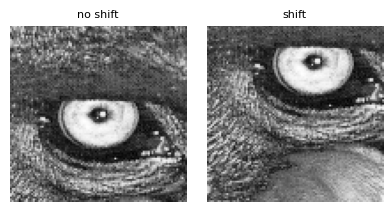
As you can observe, the coordinate shift is reflected in the bottom image.
Working with masks
In this part we will see how to use masking.
The array_grid_resampling method provides several kind of masking for both the grid and the input array.
General convention
GridR resampling functionalities uses the following convention for mask :
the mask are considered unsigned 8 bits integers taking value in {0, 1}.
a value of 0 is considered as non valid
a value of 1 is considered as valid
Grid masking
Grid masking with a raster mask
Here we use an 8 bit raster having the same shape of the grids in order to devalidate points in the grid.
To keep it simple we will demonstrate using an identity transform.
# First create identity grid
if image.ndim == 2:
    x = np.arange(0, image.shape[0], dtype=grid_dtype)
    y = np.arange(0, image.shape[1], dtype=grid_dtype)
xx, yy = np.meshgrid(x, y)
We define the mask as following :
the first 10 lines and last 20 lines are masked
the first 30 columns and last 40 columns are masked
a 80x80 window positionned at the grid center are masked
Please note the mask applies to the grid and not to the input image.
By convention, the mask is considered binary. A value of 0 corresponds to a masked cell, a value of 1 corresponds to a valid cell.
# setting a mask to devalidate margins and center
grid_mask_valid_value = 1
grid_mask_invalid_value = 0
# the final multiplication here is not necessary but we keep it to show the mechanic
grid_mask = np.ones(xx.shape, dtype=np.uint8) * grid_mask_valid_value
# masked pixels are positiv ones
grid_mask[0:10] = grid_mask_invalid_value
grid_mask[-20:] = grid_mask_invalid_value
grid_mask[:,0:30] = grid_mask_invalid_value
grid_mask[:,-40:] = grid_mask_invalid_value
# devalidate center
grid_mask[image.shape[0]//2-40:image.shape[0]//2+40, image.shape[1]//2-40:image.shape[1]//2+40] = grid_mask_invalid_value
The nodata_out is used to set the output value affected by the masking operation.
# Lets call the grid resampling
array_out, mask_out = array_grid_resampling(
        interp="cubic",
        array_in=array_in,
        grid_row=yy,
        grid_col=xx,
        grid_resolution=(1,1),
        array_out=None,
        win=None,
        array_in_mask=None,
        grid_mask=grid_mask,
        grid_mask_valid_value=grid_mask_valid_value,
        array_out_mask=True,
        nodata_out=0,
        )
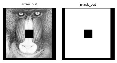
As in the previous example, we pass True to the function to obtain the validity mask output. We then check that it aligns correctly with the grid mask.
Masking with an inplaced grid nodata value
In this case, we avoid providing an additional mask, primarily to limit memory usage.
The array_grid_resampling method allows specifying a grid_nodata parameter, which is used to invalidate grid cells.
Cells in the grid whose values match this nodata value (within a fixed absolute tolerance of 1e-5) are treated as masked.
Providing a non-None value for grid_nodata activates the masking mechanism.
Note that it is not necessary to assign the nodata value to both grid coordinate arrays (row and column); setting it in either one is sufficient for the corresponding cell to be considered masked.
# Set a nodata value
grid_nodata = -999.
# Apply it to a window of the grid
yy[50:200,100:350] = grid_nodata
# Lets call the grid resampling
# Spoiler alert: this will fail !
try:
    array_out, _ = array_grid_resampling(
            interp="cubic",
            array_in=array_in,
            grid_row=yy,
            grid_col=xx,
            grid_resolution=(1,1),
            array_out=None,
            win=None,
            array_in_mask=None,
            grid_nodata=grid_nodata,
            grid_mask=grid_mask,
            grid_mask_valid_value=grid_mask_valid_value,
            array_out_mask=None,
            nodata_out=0,
            )
except ValueError as e:
    display(e)
ValueError('Only one of `grid_mask` or `grid_nodata` may be provided, not both.')
The call failed, and the ValueError exception provides the reason: both masking modes, grid_mask and grid_nodata, cannot be used simultaneously.
# Lets remove the grid_mask parameter's definition
array_out, _ = array_grid_resampling(
        interp="cubic",
        array_in=array_in,
        grid_row=yy,
        grid_col=xx,
        grid_resolution=(1,1),
        array_out=None,
        win=None,
        array_in_mask=None,
        grid_nodata=grid_nodata,
        grid_mask=None,
        grid_mask_valid_value=None,
        array_out_mask=None,
        nodata_out=0,
        )
Effect of Grid Resolution on Grid Masking
Both the raster mask and the invalid_value grid mask remain consistent with the sampling of the grid.
When the resolution differs from 1 in a given direction, interpolation must occur within each grid cell — that is, within the mesh defined by four neighboring grid nodes. In such cases, if at least one non-zero weighted node of the mesh is masked, the interpolated result is marked as invalid. This results in nodata values in the resampled image and corresponding invalid entries (value 0) in the output mask.
Let’s illustrate this behavior by zooming in on a small region.
# create identity grid on the eye
if image.ndim == 2:
    x = np.arange(130, 220, dtype=grid_dtype)
    y = np.arange(30, 100, dtype=grid_dtype)
xx, yy = np.meshgrid(x, y)

resolution = np.asarray((2,3))

# lets define the mask using grid_nodata
grid_nodata = -99999
yy[30, 35] = grid_nodata

array_out, mask_out = array_grid_resampling(
        interp="cubic",
        array_in=array_in,
        grid_row=yy,
        grid_col=xx,
        grid_resolution=tuple(resolution),
        array_out=None,
        win=None,
        array_in_mask=None,
        grid_nodata=grid_nodata,
        array_out_mask=True,
        nodata_out=0,
        )
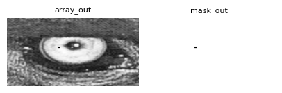
To invalidate a specific grid position, we’ve configured the input (30, 35). This grid coordinate directly corresponds to the (60, 105) output position in the output coordinate system.
print(mask_out[60-2:60+3,105-3:105+4])
print(f"Number of masked data : {np.where(mask_out==0)[0].shape}")
[[1 1 1 1 1 1 1]
 [1 0 0 0 0 0 1]
 [1 0 0 0 0 0 1]
 [1 0 0 0 0 0 1]
 [1 1 1 1 1 1 1]]
Number of masked data : (15,)
The masked area, as illustrated, exceeds a single pixel due to a resolution factor of 2 for rows and 3 for columns. The displayed array is centered on the position of the invalid grid node. Notably, this invalidation propagates to its immediate neighborhood, but exclusively for interpolated values where its weight is non-zero.
For clearer comprehension, in the schema below, an x denotes an invalid grid node, an o represents other grid nodes, and both - and * signify oversampled positions. It’s crucial to note that only the * positions utilize the x (invalid grid node) in their bilinear interpolation calculations.
 o - - o - - o
 - * * * * * -
 o * * x * * o
 - * * * * * -
 o - - o - - o
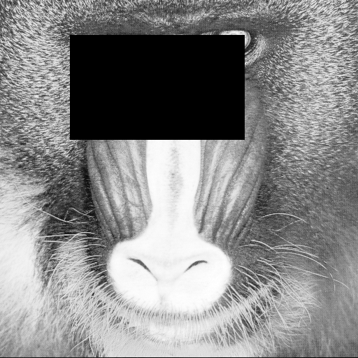
Input Array masking
Array masking with a raster mask
Here we use an 8 bit raster having the same shape of the input array in order to devalidate points in the input array.
Basically if input data is devalidate, interpolation that involves those data must be considered as not valid resulting in output valued to nodata_out and the optional array_out_mask set to 0 instead of 1.
To keep it simple we will demonstrate using a simple zoom transformation transform.
array_in_mask = np.ones(array_in.shape, dtype=np.uint8)
masked_pos = (60, 160)
array_in_mask[*masked_pos] = 0
# In order to check the good interpolation we will also set the array_in to hold an aberrant value
save_array_in = array_in[*masked_pos]

# Create a grid centered on the masked position
y = masked_pos[0] + np.linspace(-3, 3, 100)
x = masked_pos[1] + np.linspace(-3, 3, 100)
xx, yy = np.meshgrid(x, y)

# First compute a
array_out_womask_truth, _ = array_grid_resampling(
        interp="cubic",
        array_in=array_in,
        grid_row=yy,
        grid_col=xx,
        grid_resolution=(1,1),
        array_out=None,
        nodata_out=0,
        )

# Second compute without array masking to watch the effect of the non masked aberrant value
array_in[*masked_pos] = 1e7

array_out_womask, _ = array_grid_resampling(
        interp="cubic",
        array_in=array_in,
        grid_row=yy,
        grid_col=xx,
        grid_resolution=(1,1),
        array_out=None,
        array_out_mask=True,
        nodata_out=0,
        )

aberrant_radiation = np.zeros(array_out_womask.shape)
aberrant_radiation[np.where(array_out_womask - array_out_womask_truth != 0)] = 1

# Recompute with the mask
array_out, mask_out = array_grid_resampling(
        interp="cubic",
        array_in=array_in,
        grid_row=yy,
        grid_col=xx,
        grid_resolution=(1,1),
        array_in_mask=array_in_mask,
        array_out=None,
        array_out_mask=True,
        nodata_out=150, # Here we set nodata_out to 150 in order to have some texture for the display
        )
# restore array_in
array_in[*masked_pos] = save_array_in
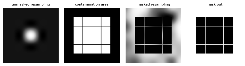
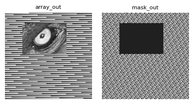
We have several plots to analyze here.
The first plot reveals what happens when the anomalous value is not masked. While the 8-bit display dynamic range prevents us from fully appreciating the valid interpolation, this plot effectively showcases the influence of an anomalous value (exaggerated for illustrative purposes) on the interpolation process.
The second plot, a binary representation, indicates where the anomalous value “spreads” or “irradiates.” Interestingly, some unaffected lines can be seen traversing the “irradiated” zone.
The third plot demonstrates the outcome when the anomalous value is successfully masked. We can see a clear correspondence between the no-data pixels and the “irradiated” area.
Lastly, the final plot presents the output validity mask, confirming its consistency with our earlier findings.
# min and max indices of masked data
upper_left = np.min(np.where(mask_out==0), axis=1)
lower_right = np.max(np.where(mask_out==0), axis=1)
print(f'upper left corner of masked data : {upper_left}')
print(f'lower right corner of masked data : {lower_right}')

# corresponding grid coordinates
print(f'masked data upper left corner grid coordinates : {yy[*upper_left], xx[*upper_left]}')
print(f'masked data lower right corner grid coordinates : {yy[*lower_right], xx[*lower_right]}')
upper left corner of masked data : [17 17]
lower right corner of masked data : [82 82]
masked data upper left corner grid coordinates : (np.float64(58.03030303030303), np.float64(158.03030303030303))
masked data lower right corner grid coordinates : (np.float64(61.96969696969697), np.float64(161.96969696969697))
The optimized bicubic interpolator uses a spatial support of ±2 around the target coordinates. This directly explains the masked area’s boundaries: row indices [58,62] and column indices [158,162].
Now, let’s discuss the unmasked lines that cross the invalid area. To do this, we will plot the grid coordinates, differentiating between the valid and invalid ones.
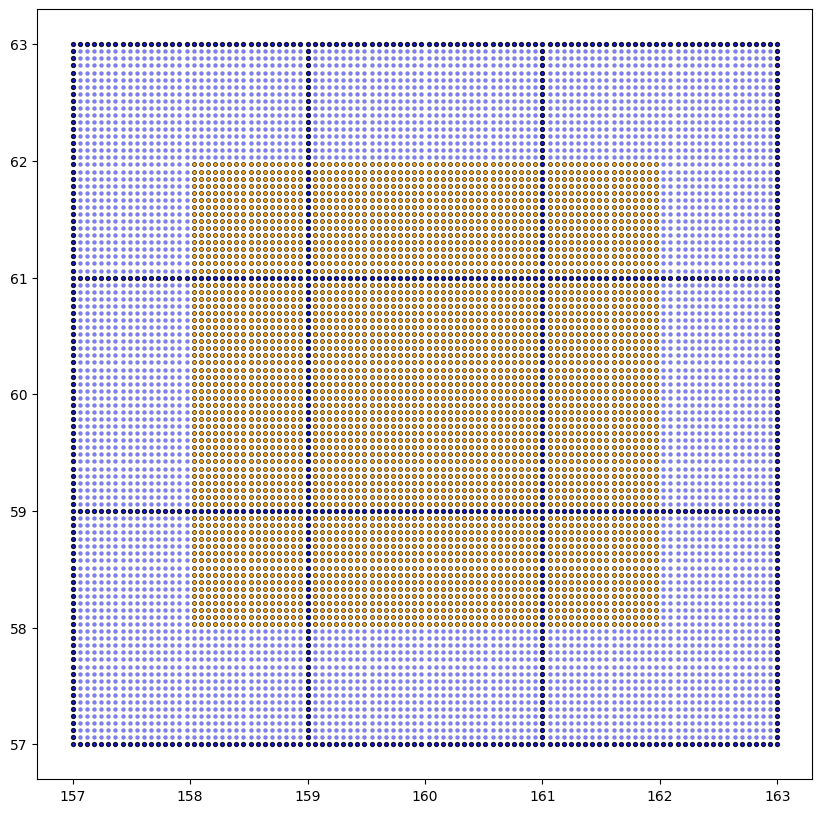
We’ve used a distinct style in the plot above to highlight coordinates that fall on exact integer values. This specific scenario, where we have whole integer coordinates within our grid, serves to prove that the GridR implementation aligns correctly with the “irradiated” area. It also shows that it avoids inadvertently masking pixels that should remain unmasked.
What makes these integer coordinate positions unique? For these particular points, the subsequent interpolation process can utilize a directly available value in at least one direction, meaning no actual interpolation is required along that axis. In these instances, the neighboring points that would normally contribute to the interpolation—especially any anomalous ones—are effectively bypassed. Their associated coefficients are set to zero, which then yields a perfectly valid interpolated value.